Each location in this layer is associated with a land cover class value as well as a parcel use code.
This document describes the characteristics of both elements, and the usefulness and convenience of the combined product.
Download the MassGIS 2016 Land Use/Land Cover Data data
Although both land cover and land use information are included, each of these aspects can be accessed independently, or in interesting and useful combinations with one another. For instance, a user can simply display impervious surfaces (land cover), or commercial parcels (land use). In combination, it is possible to display and measure the portions of the commercial parcels that are covered by impervious surfaces or the portions of residential parcels used as developed open space.
This layer is the result of a cooperative project between MassGIS and the National Oceanic and Atmospheric Administration’s (NOAA) Office of Coastal Management (OCM). Funding was provided by the Mass. Executive Office of Energy and Environmental Affairs.
MassGIS stores the data as a single statewide polygon feature class named LANDCOVER_LANDUSE_POLY in the spatial reference of NAD_1983_Contiguous_USA_Albers (EPSG: 5070).
Data Development
The following sections describe the development and features of the two components, land cover and land use, as well as the final combined dataset.
Land Cover
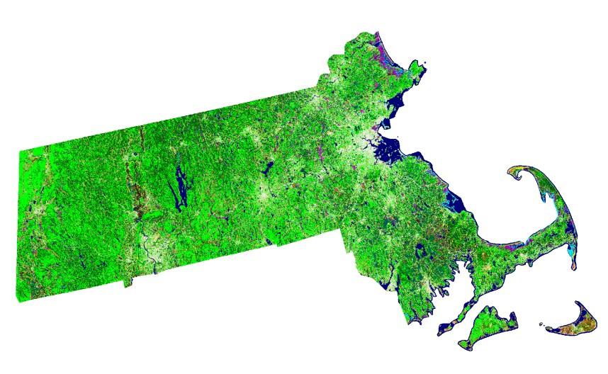
The thematic land cover dataset was created in raster format by NOAA's Coastal Change Analysis Program (C-CAP). C-CAP has produced numerous standardized land cover products which are included in the National Land Cover Database. These products are used in numerous ways to assess urban growth, inventory wetlands, coastal intertidal areas, and adjacent uplands, and delineate wildlife habitat to monitor changes in these areas. This information helps in the understanding of the landscape's response to natural and human-caused changes. OCM worked in close coordination with MassGIS to produce the land cover. OCM delivered the data to MassGIS in an Albers projection.
This 2016 land cover information was initially developed as a 1-meter, 6-category draft raster derived from 2016 USDA National Agricultural Imagery Program (NAIP) aerial multispectral imagery. Classes were impervious, bare, grass, shrub, tree, and water. Additional reference data were used to create this 19-class version, including: 2016 WorldView multispectral satellite imagery, lidar-based terrain elevation data, 2016-era 2D structures data, and other ancillary data such as MassDOT Roads, MassDEP Wetlands, etc. The wetlands in the final land cover product are exclusively from the C-CAP program and will differ from the MassDEP Wetlands data.
The land cover information in this product are consistent with C-CAP’s High-Resolution Land Cover Classification Scheme. See descriptions of the land cover classes that were used.
See general information about C-CAP High-Resolution Land Cover.
The classes used in the C-CAP 2016 Massachusetts High-Resolution Land Cover product are as follows:
| Class Number | Class Name |
|---|---|
| 2 | Impervious |
| 5 | Developed Open Space |
| 6 | Cultivated Land |
| 7 | Pasture/Hay |
| 8 | Grassland |
| 9 | Deciduous Forest |
| 10 | Evergreen Forest |
| 12 | Scrub/Shrub |
| 13 | Palustrine Forested Wetland (C-CAP) |
| 14 | Palustrine Scrub/Shrub Wetland (C-CAP) |
| 15 | Palustrine Emergent Wetland (C-CAP) |
| 16 | Estuarine Forested Wetland (C-CAP) |
| 17 | Estuarine Scrub/Shrub Wetland (C-CAP) |
| 18 | Estuarine Emergent Wetland (C-CAP) |
| 19 | Unconsolidated Shore |
| 20 | Bare Land |
| 21 | Open Water |
| 22 | Palustrine Aquatic Bed (C-CAP) |
| 23 | Estuarine Aquatic Bed (C-CAP) |
Data for Massachusetts do not exist for all classes within the C-CAP scheme. There are no areas representing the following classes:
| Class Number | Class Name |
|---|---|
| 1 | Unclassified |
| 11 | Mixed Forest |
| 24 | Mixed Forest |
| 25 | Perennial Ice/Snow |
| 26 | Dwarf Scrub - Alaska specific class |
| 27 | Sedge/Herbaceous |
| 28 | Moss - Alaska specific |
Developed classes have been altered to exclude the percentage breakdown of impervious surfaces since the breakdown is not appropriate for high resolution mapping. Therefore classes 2 (Developed High Intensity), 3 (Developed Medium Intensity), and 4 (Developed Low Intensity) are reduced to: Class 2 (Impervious).
Land Cover Classification
The initial 6-class land cover product as well as the 19-class final product were developed using Geographic Object-Based Image Analysis (GEOBIA) and an expert image analysis processing framework.
Classification involved taking each image to be classified and grouping the pixels based on spectral and spatial properties into regions of homogeneity called objects. The resulting objects are the primary units for analysis. Additionally, these objects introduce additional spectral, shape, textural and contextual information into the mapping process and are utilized as independent variables in a supervised classification. Each object is labeled using a Random Forest Classifier which is an ensemble version of a Decision Tree. Training data for the initial 6 classes (Herbaceous, Bare, Impervious, Water, Forest and Shrub) were generated through photo interpretation. The resulting Random Forest model was applied to the input data sets to create the initial automated map.
The following are some details about the creation of land cover classes:
Water Refinement
Commission and omission errors associated with the Water class were addressed through manual interpretation and clean-up in ERDAS IMAGINE. Once the review and edits were complete, the refined Water class was incorporated back into the land cover dataset.
Unconsolidated Shore
Unconsolidated substrate features were extracted primarily through unsupervised classification and manual editing in ERDAS IMAGINE. This process relied on the USGS Color Orthoimagery (2013/2014) as a primary data source since it was collected at a lower tidal stage relative to other available imagery. Once these features were inserted into the land cover additional object based clean up algorithms were applied.
Agriculture
Cultivated land and Pasture/Hay features were incorporated into the grassland category of the initial land cover product through a modeling process which relied on multiple dates of imagery as well as the 2005 statewide land use data set. Manual edits were made based on feedback from local experts.
C-CAP Wetlands
C-CAP Wetlands were derived through a modeling process which used ancillary data such as Soils (SSURGO), the National Wetlands Inventory (NWI) and topographic derivatives. Forest, shrub and grassland objects within the initial land cover that exhibited hydric characteristics based on the input ancillary layers were designated to their appropriate C-CAP wetland category. The process relied mainly on the NWI to determine palustrine and estuarine distinctions.
Open Space Developed
Managed grasses and other low-lying vegetation associated with development were derived using information in the 2005 statewide land use data set. Grassland features in the land cover data that intersected selected land use polygons were designated as Open Space Developed (OSD). To capture OSD features that have appeared since the 2005 land use data was developed, polygons with land use codes that were likely candidates for change were analyzed for the presence of impervious surface based on the 2015 land cover. If the polygon was occupied by a certain percent of impervious surface, the associated grass pixels were changed to Open Space Development. Additional cleanup was performed to remove speckle and slivers.
Developed features were mapped with a 0.10-acre minimum mapping unit (MMU), and non-developed (natural) areas have an MMU of 0.25 acres. Features smaller than these defined MMUs were allowed if generally seen as beneficial.
The land cover data was delivered as an uncompressed thematic raster file (.img) in which each individual pixel element is labeled with a land cover class value.
Quality assurance tests for logical consistency indicate that all row and column positions in the selected latitude/longitude window contain data. Conversion and integration with vector files indicate that all positions are consistent with earth coordinates covering the same area. Attribute files are logically consistent.
Raster information and Spatial Reference:
| Item | Description |
|---|---|
| Projection | Albers Conical Equal Area |
| Spheroid Name | GRS 1980 |
| Spheroid Axis | 6378137.000000, 6356752.314140 |
| Datum Name | NAD83 |
| Datum Parameters | 0.0, 0.0, 0.0, 0.0, 0.0, 0.0, 0.0 |
| Latitude of 1st standard parallel | 29.5 N |
| Latitude of 2nd standard parallel | 45.5 N |
| Longitude of central meridian | 96.0 W |
| Latitude of origin of projection | 23.0 N |
| False easting at central meridian | 0.0 meters |
| False northing at origin | 0.0 meters |
| EPSG Code | 5070 |
| Pixel Size X & Y | 1.0 |
| Unit | meters |
Validation of The Land Cover Classification
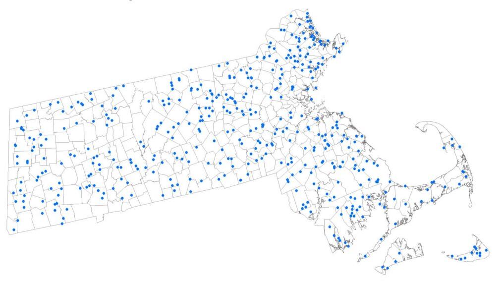
The quality of the result was checked by randomly sampling the land cover map at numerous locations and comparing the classification result to the actual “true” class, determined by a visual interpretation of the aerial imagery.
NOAA sampled a total of 446 points distributed across the state using a stratified random sampling scheme, with a minimum target sample of 10 points per class. A few of the rarer categories did not meet this minimum threshold target.
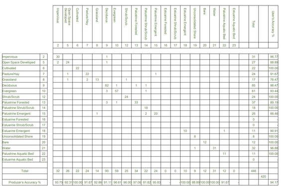
Land Cover Accuracy Assessment – Error Matrix
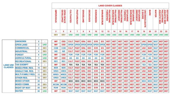
Example of matrix used to reduce number of combined land cover / use categories for mapping.
Aside from the wetlands classes, the rule applied here is:
- If both classes are developed (DEV) or if both classes are undeveloped (UND), the land use class is mapped.
- If one class is developed, and the other is undeveloped, the land cover class is mapped.
The results of this comparison were assembled into an error matrix, which was used to calculate a variety of accuracy measures.
In the table, the columns represent the reference data or the data that is known to be correct. The rows represent the mapped classes from the aerial imagery. For example, 32 points were observed to be on Impervious surfaces (column total), and there were 31 points mapped as Impervious (row total).
The diagonal elements of the error matrix represent instances where the real class agreed with the mapped class. The sum of the diagonal elements is the number of correctly classified points (420), while the total number of reference sites is 446. The proportion of the reference sites that were mapped correctly is a measure of overall accuracy. 420/446 = 0.9417.
Errors are represented by values outside the diagonal.
- Producer's Accuracy is the probability that real features on the ground are correctly shown on the classified map. Number of correctly classified sites in each category by the number of sites that are really that class. There were 82 points mapped as Deciduous out of 90 points that should have been mapped that way. Producer’s accuracy is 82/90 = 0.9111 for Deciduous.
- Errors of Omission are sites that are incorrectly mapped. For example, for Deciduous: 8 sites were incorrectly classified out of 90, so the error of omission for Deciduous = 8/90 (about 9%).
- User's Accuracy measures how often a mapped value at a point corresponds to that same class on the ground. The number of correctly classified points in each category divided by the total number of points that were in that class on the map. There were 85 points mapped as Deciduous. 85/90 or about 96.5% were mapped correctly.
- Errors of Commission (“False positives”) Three points were mapped as Deciduous, but these should have been mapped in other categories. 3/85 is about 3.5% errors of commission for Deciduous.
Other statistics can be derived from the table.
The accuracy of each class is summarized below:
| Class | Producer's Accuracy | User's Accuracy |
|---|---|---|
| Impervious | 93.7% | 96.8% |
| Open Space Developed | 92.3% | 88.9% |
| Cultivated | 100% | 100% |
| Pasture/Hay | 91.7% | 91.7% |
| Grassland | 92.9% | 76.5% |
| Deciduous Forest | 91.1% | 96.5% |
| Evergreen Forest | 96.6% | 93.4% |
| Shrub/Scrub | 96.0% | 100% |
| Palustrine Forested Wetland (C-CAP) | 97.1% | 89.2% |
| Palustrine Shrub/Scrub Wetland (C-CAP) | 81.8% | 100% |
| Palustrine Emergent Wetland (C-CAP) | 95.8% | 88.5% |
| Estuarine Forested Wetland (C-CAP) | N/A | N/A |
| Estuarine Shrub/Scrub Wetland (C-CAP) | N/A | N/A |
| Estuarine Emergent Wetland (C-CAP) | 100% | 90.9% |
| Unconsolidated Shore | 88.9% | 100% |
| Bare Land | 100% | 100% |
| Water | 100% | 96.9% |
| Palustrine Aquatic Bed (C-CAP) | 91.7% | 100% |
| Estuarine Aquatic Bed (C-CAP) | N/A | N/A |
The number of correctly classified sites (the sum of the diagonal elements) = 420. The total number of reference sites = 446. According to the accuracy assessment performed by NOAA Office for Coastal Management staff, the overall accuracy of this product = 420/446 = 94.2%.
Estuarine Forested Wetland (C-CAP), Estuarine Shrub/Scrub Wetland (C-CAP), and Estuarine Aquatic Bed Wetland (C-CAP) were not sampled at all due to the relatively low total area of those classes. Additionally, Unconsolidated Shore ended up with only 9 sample locations. Ideally, a larger number of samples would have been included.
The correct land cover classification was determined through analyst interpretation of the imagery used in creating the map, as well as possible references to Google Earth to reference additional dates/seasons of imagery for that location. All points were interpreted by two analysts, plus a third who made a final determination when there was not agreement on the call. All analysts could identify both a primary “call” as well as a fuzzy call if the point location caused any level of confusion as to what the land cover category was.
Land Use from Property Type Classification Codes
The land use component of the data layer is represented by the Property Type Classification Code associated with each parcel in MassGIS' Standardized "Level 3" Parcels layer. These "use codes" come from the Mass. Department of Revenue Division of Local Services (DLS), along with custom use codes some municipalities include in their parcel data.
Creation of the 2016 Statewide "Patchwork" Parcel Map
MassGIS created a statewide standardized parcel map with the following attributes:
- USE_CODE
- FY (FISCAL YEAR)
- POLY_TYPE
- TOWN_ID
- GEN_CODE
It was intended to fix the time of the parcel data as close as possible to the time of the 2016 NAIP imagery.
Since parcel data complying with Level 3 of the MassGIS standard was not available from every municipality for the year 2016, some information was selected from a different year to use data as close to the year 2016 as possible.
Priority was given to more recent submissions as it is less detrimental to include a developed USECODE from a later Fiscal Year that co-exists with undeveloped landcover than it is to have development appear in landcover where an undeveloped assessor USECODE is assigned.
Data was selected and added to the product by searching for data applying the following rule: If Fiscal Year (FY) 2016 data was available, it was used. Otherwise, data was used from other years in the following order: 2017 (+1), 2015 (-1), 2018 (+2), 2014 (-2), 2013 (-3), 2012 (-4), 2011 (-5).
Fiscal year values were retained in the final product to help indicate relative reliability of the USECODE.
Stacked Polygons
The resolution of the Fiscal Year issue resulted in a view where the assessor attributes associated with a parcel were joined to it, but there remained numerous parcels with more than one associated assessor record.
These appeared as "stacked" polygons, each joined to a single record. This situation, where there was more than one land use code that can be assigned to a location, was resolved in a variety of ways to reasonably represent the land use for each parcel.
To eliminate many of the stacked polygons that were functionally redundant, a “Delete Identical” geoprocessing operation was run on the parcel product to remove stacked polygons that share the same LOC_ID and USE_CODE.
What remained were stacked parcel polygons that linked to multiple assessing records with different USECODEs. These were resolved in several ways:
All polygons with USECODE values of 995 and 996 (commonly owned condominium open space) that coexist with developed condominium USECODEs (commonly 102) were removed from the product.
Then all non-unique LOC_ID values in the parcels were identified. These represented stacked polygons with multiple distinct USECODEs and their resolution required applying some general “rules of thumb”.
For example, several stacked polygons, where some had a residential condominium code and the others had a commercial condominium code, were replaced by a single polygon with a mixed USECODE representing both residential and commercial use.
However, there are two possible codes that can represent mixed residential and commercial: 013 and 031. "0" indicates mixed, "1" indicates Residential, and "3" indicates Commercial. Since the first non-zero number should represent the use which is more dominant, a code of "013" means: "Mixed use Residential with Commercial (primarily Residential)", and "031" means: "Mixed use Commercial with Residential (primarily Commercial)".
A field named “LAND_SF” represents the square footage area for a property, and the LAND_SF values associated with the residential codes and those associated with the commercial codes were aggregated and compared to determine which use was dominant.
It was not uncommon to find maybe 10 Residential condominium records and only one or two Commercial condominium records, so the majority of these were coded "013".
Another rule of thumb: When two codes represent the same kind of general use, eliminate one of the polygons, and defer to non-tax-exempt codes when they coexist with tax exempt codes.
When multiple use codes were associated with a single parcel, the parcel was sometimes classified with an appropriate "Mixed Use" code (i.e. a residential code 101 and a commercial code 340 would be replaced by a single polygon with a "Multi Use" code of 013 or 031).
All non-unique LOC_IDs that link to a developed use code and an undeveloped use code will have the polygon with the undeveloped use code removed from the product. (e.g. 101 & 130: Remove the polygon with the USECODE = 130).
Any non-unique LOC_ID values that link to two or more developed use codes were reclassified as “MIXED USE”, deleting the extra stacked polygons and optionally replacing the remaining polygon’s use code with a replacement use code representing mixed use in arbitrary fashion. (i.e. a property with a single-family house and a family-owned auto repair business run out of the garage has a 101 and 332 use code assigned in different tax records. A replacement use code of 013 or 031 can optionally be recorded in the remaining polygon’s use code).
Residential condominiums were assigned to MULTIFAMILY RESIDENTIAL.
In a few cases, new USECODEs were recently created, and descriptions were not available in the statewide use code lookup table. In these cases, an educated guess was made based on the single-digit code represented by the first number in a 3-digit code or the 1 st or 2 nd digit in a 4-digit code depending on whether prepended 0’s were used or not. The guess was informed by the DOR classification code documentation.
A use classification of “ROW” for parcels with POLY_TYPE in [“ROW”, “RAIL_ROW”, and “PRIV_ROW”] was populated in the parcel product. A use classification of “WATER” for parcels with POLY_TYPE = “WATER” was populated in the parcel product. Any other parcel that did not link to an assessor record was assigned a use classification of “UNKNOWN”.
Attribute “FY_OF_INTEREST” represents the FY value in the assessor tables of the data for each town ultimately deemed most appropriate for the baseline and incorporated into the product.
Cities and towns in Massachusetts have created customized USE_CODES based on the standard, so that there are over 1600 unique values for USE_CODE in the parcel data. As an alternative, the attribute “GEN_CODE” was added to BASELINE_TAXPAR_2016_FINAL and populated with generalized values using a table named MASSGIS.BASELINE_GEN_USE_LOOKUP. This table contains the generalized use descriptions and an associated generalized USE_CODE.
Also used was a table called MASSGIS.BASELINE_2016_GEN_USE_LOOKUP. This table contains a record for every USE_CODE value in the BASELINE_TAXPAR_2016_FINAL product along with its generalized code and generalized description.
The generalized codes and descriptions are as follows:
| GEN_CODE | DESCRIPTION |
|---|---|
| 0 | UNKNOWN |
| 2 | OPENLAND |
| 3 | COMMERCIAL |
| 4 | INDUSTRIAL |
| 6 | FOREST |
| 7 | AGRICULTURAL |
| 8 | RECREATIONAL |
| 9 | EXEMPT (TAX-EXEMPT) |
| 10 | MIXRES (MIXED USE, PRIMARILY RESIDENTIAL) |
| 11 | RESSINGLE (SINGLE-FAMILY RESIDENTIAL) |
| 12 | RESMULTI (MULTI-FAMILY RESIDENTIAL) |
| 13 | RESOTHER (OTHER RESIDENTIAL) |
| 20 | MIXOTHER (MIXED USE, OTHER) |
| 30 | MIXCOM (MIXED USE, PRIMARILY COMMERCIAL) |
| 55 | ROW (RIGHT-OF-WAY) |
| 88 | WATER |
WATER and the various ROW (Right of way) poly types were assigned GEN_CODE’s of 88 and 55 codes respectively.
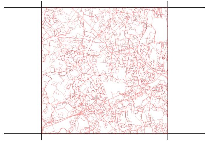
Combined Land Cover – Land Use Data
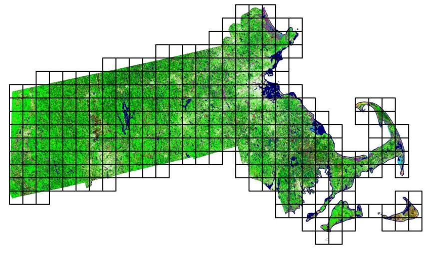
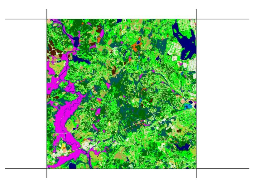
For efficient processing and distribution, MassGIS split up the statewide land cover raster into 291 smaller, regularly sized and spaced tiles, each 10km by 10km (10,000 x 10,000 pixels).
The Create Fishnet tool produced a polygon index that precisely fit the tiles. The tiles were identified with a TILENAME value based on row and column position. For example, TILENAME “R07C17” identifies the tile in row 7, column 17. The index is named LANDCOVER_USE_INDEX_POLY. Aside from TILENAME, the other field is SHP_LINK, which stores a link to download a zipped land cover-land use shapefile for each tile.
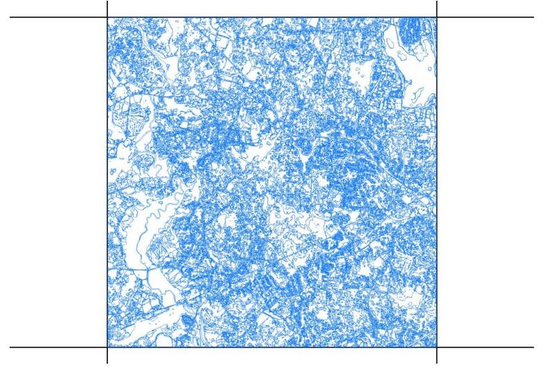
In order to match the data model of the land use ahead of combining the two datasets, each land cover image was converted to a polygon shapefile ("vectorization") using a Raster to Shapefile model in ERDAS IMAGINE. This method preserves the thematic attributes and simplifies the polygons very slightly.
MassGIS carried out the following steps in ArcGIS 10.6.1:
- Reprojected the land use polygons from Massachusetts State Plane to the same Albers projection of the land cover.
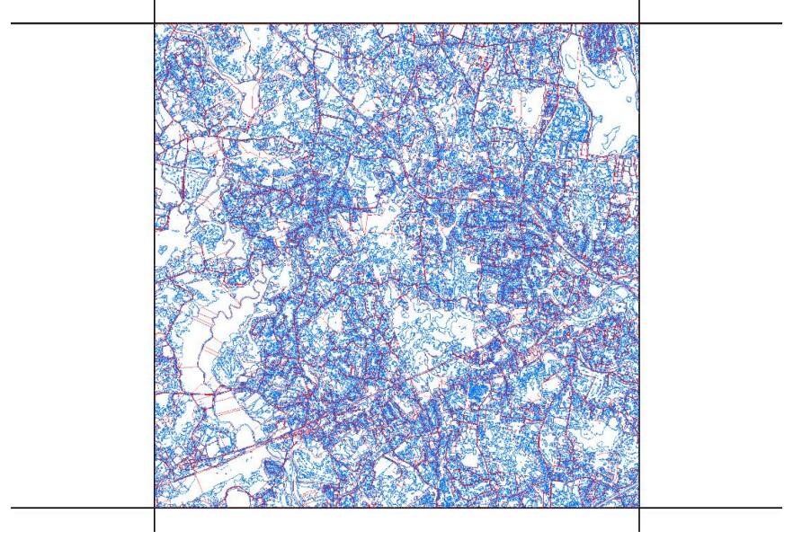
- Used the Identity tool to geometrically combine the land cover polygons with the dissolved parcel data to produce a land cover-land use feature class for each tile.
- Checked and repaired the geometry of the Identity output.
- Converted all multipart polygons to single-part polygons in the Identity output
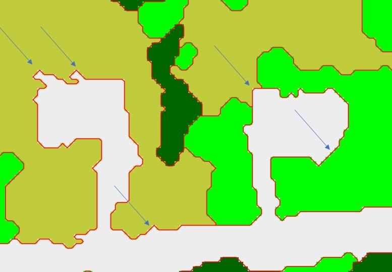
The Identity created numerous very small polygons because the two components (land cover and land use) were not spatially correlated. To preserve the input data, MassGIS decided not to eliminate polygons or perform any other cartographic refinement at this point. Users can easily perform these operations if desired.
The fields in the final land cover-land use data are:
| Field | Type | Description |
|---|---|---|
| COVERNAME | Char / 50 | Land cover class name |
| COVERCODE | Integer / 5 | Land cover class code |
| USEGENNAME | Char / 50 | Generalized land use name |
| USEGENCODE | Integer / 5 | Generalized land use code |
| USE_CODE | Char / 4 | Detailed parcel use code |
| POLY_TYPE | Char / 15 | Parcel polygon type |
| FY | Integer / 5 | Fiscal year of parcel data |
| TOWN_ID | Integer / 5 | City/Town ID (1-351). Polygons with a TOWN_ID of zero are in areas where the land cover occurs offshore. |
| TILENAME | Char / 6 | Index tile name used for shapefile distribution |